Image Classification Model for Rock-Paper-Scissors

Building an Image Classification Model for Rock-Paper-Scissors Using Deep Learning

Introduction

In today's rapidly evolving digital era, machine learning technology has become one of the most crucial fields in data processing. One fascinating application of machine learning is image classification, where models are programmed to recognize and categorize images based on their content. In this article, we will explore the complex process of building and evaluating an image classification model using deep learning methods. Specifically, we will focus on developing a model capable of accurately distinguishing between hand gestures depicting rock, paper, and scissors. Through a carefully crafted series of steps, we will discuss everything from importing data to model evaluation, providing deep insights into the workings of modern machine learning techniques. Building an image classification model is the first step towards more advanced applications such as object detection, facial recognition, and even autonomous vehicles. With the ability to understand and interpret the visual world like humans, image classification models can be used in various industries, including security surveillance, pattern recognition, medical diagnostics, and much more.

Dataset Collection

The dataset used in this project comes from the Dicoding class. Dicoding provides diverse and high-quality datasets to support learning in programming and technology fields. The rockpaperscissors dataset used in this article consists of images depicting hand gestures of rock, paper, and scissors. Using this dataset provides advantages in data consistency and quality, which are crucial in training accurate and reliable machine learning models.

1. Import Library

            import tensorflow as tf
            from tensorflow.keras.preprocessing.image import ImageDataGenerator
            from tensorflow.keras.models import Sequential
            from tensorflow.keras.layers import Conv2D, MaxPooling2D, Flatten, Dense
            from tensorflow.keras.optimizers import RMSprop
            from tensorflow.keras.callbacks import EarlyStopping, ModelCheckpoint
            import matplotlib.pyplot as plt
            import zipfile
            import os
            from sklearn.metrics import classification_report, confusion_matrix
            from keras.preprocessing import image
            from datetime import datetime, timedelta
            from tensorflow.keras.callbacks import EarlyStopping
            

Import TensorFlow

import tensorflow as tf

The first step in the machine learning model development process is to import the TensorFlow library. TensorFlow is a powerful open-source machine learning framework developed by Google. It provides a comprehensive ecosystem of tools, libraries, and community resources for building and deploying machine learning models.

Import ImageDataGenerator

from tensorflow.keras.preprocessing.image import ImageDataGenerator

The ImageDataGenerator class from TensorFlow Keras API is used for data augmentation and preprocessing of images during model training. Data augmentation techniques such as rotation, scaling, and flipping can help improve the robustness and generalization of the trained model.

Import Sequential Model

from tensorflow.keras.models import Sequential

The Sequential model from TensorFlow's Keras API is a linear stack of layers. It allows for easy and intuitive building of deep learning models by simply adding layers in sequence.

Import Layers

from tensorflow.keras.layers import Conv2D, MaxPooling2D, Flatten, Dense

Various layer types such as convolutional, pooling, flattening, and dense (fully connected) layers are essential components of neural network architectures. These layers are imported from TensorFlow's Keras API for building the model.

Import Optimizers

from tensorflow.keras.optimizers import RMSprop

Optimizers are algorithms used to update the weights of the neural network during training in order to minimize the loss function. RMSprop is one of the optimization algorithms available in TensorFlow, suitable for training deep neural networks.

Import Callbacks

from tensorflow.keras.callbacks import EarlyStopping, ModelCheckpoint

Callbacks are objects that can perform actions at various stages of the training process, such as stopping training early if no improvement is observed or saving the model's weights after every epoch. Here, we import EarlyStopping and ModelCheckpoint callbacks for monitoring and managing the training process.

Import Visualization Tools

import matplotlib.pyplot as plt

Matplotlib is a popular data visualization library in Python. We import it here to visualize training and evaluation metrics such as loss and accuracy.

Import Zipfile Module

import zipfile

The zipfile module in Python provides tools for creating, reading, writing, and extracting ZIP archives. It is used here to handle the extraction of dataset files.

Import Operating System Module

import os

The os module in Python provides functions for interacting with the operating system, such as reading or writing files, manipulating paths, and managing directories. It is used here for specifying file paths during dataset extraction.

Import Classification Metrics

from sklearn.metrics import classification_report, confusion_matrix

Classification metrics such as precision, recall, and F1-score are important for evaluating the performance of classification models. We import classification_report and confusion_matrix from scikit-learn for computing these metrics.

Import Image Preprocessing

from keras.preprocessing import image

The image module from Keras provides utilities for loading, preprocessing, and augmenting image data. It is used here for image preprocessing tasks such as loading images from files.

Import Date and Time Module

from datetime import datetime, timedelta

The datetime module in Python provides classes for manipulating dates and times. It is used here for time-related calculations or operations.

Import EarlyStopping Callback

from tensorflow.keras.callbacks import EarlyStopping

The EarlyStopping callback in TensorFlow is used to stop training when a monitored metric has stopped improving. It helps prevent overfitting by terminating training early when performance on the validation set begins to degrade.

2. Dataset Collection

            !wget https://github.com/dicodingacademy/assets/releases/download/release/rockpaperscissors.zip

            with zipfile.ZipFile("rockpaperscissors.zip", "r") as zip_ref:
                zip_ref.extractall("/content/")

            dataset_dir = "/content/rockpaperscissors/rps-cv-images/"
            

Next, the dataset needs to be collected to train and test the model. The dataset used in this project is the rockpaperscissors dataset provided by Dicoding. This stage includes downloading the dataset from its source and extracting the ZIP file to the correct directory.

Here are explanations for each step in the dataset collection stage:

1. Download the Dataset: First, we use the wget command to download the rockpaperscissors.zip dataset file from its source. This link directs to the GitHub repository containing the dataset. Downloading the dataset is an important initial step before we can use the data to train and test the model.
2. Extract the Dataset: After the dataset file is successfully downloaded, the next step is to extract it. In this code, we use the zipfile module to extract the ZIP file. The extractall() function is used to extract all contents of the ZIP file to the specified directory. In this case, the contents of rockpaperscissors.zip will be extracted to the /content/ directory.
3. Dataset Directory: After the dataset is extracted, we define the directory location where the dataset is stored. In this case, the dataset directory is stored in /content/rockpaperscissors/rps-cv-images/. This step is important because we will use this location to access the dataset when splitting it into training and validation data, as well as when training the model.

This stage is the initial step required in the dataset collection process to train the model. By downloading and extracting the dataset, we are ready to proceed to the next steps in building the image classification model.

3. Dataset Splitting

            train_dir = os.path.join(dataset_dir, 'train')
            val_dir = os.path.join(dataset_dir, 'val')

            os.makedirs(train_dir, exist_ok=True)
            os.makedirs(val_dir, exist_ok=True)

            for label in ['rock', 'paper', 'scissors']:
                os.makedirs(os.path.join(train_dir, label), exist_ok=True)
                os.makedirs(os.path.join(val_dir, label), exist_ok=True)
            

Firstly, this code creates two new directories: one for the training data ('train_dir') and one for the validation data ('val_dir'). These directories will be used to store the images used in the training and validation processes of the model. The os.makedirs() function is used to create directories, with the parameter exist_ok=True to avoid errors if the directory already exists. The os.path.join() function is used to combine the dataset_dir (main dataset directory) with the desired sub-directory names.

            datagen = ImageDataGenerator(
                rescale=1./255,
                rotation_range=20,
                horizontal_flip=True,
                shear_range=0.2,
                zoom_range=0.2,
                validation_split=0.4
            )
            

This code uses the ImageDataGenerator from the Keras module to prepare the training and validation data by performing image augmentation such as rotation, horizontal flipping, shear, and zoom. The parameter validation_split=0.4 indicates that 40% of the entire data will be allocated as validation data.

            train_generator = datagen.flow_from_directory(
                dataset_dir,
                target_size=(150, 150),
                batch_size=32,
                class_mode='categorical',
                subset='training',
                classes=['rock', 'paper', 'scissors']
            )

            val_generator = datagen.flow_from_directory(
                dataset_dir,
                target_size=(150, 150),
                batch_size=32,
                class_mode='categorical',
                subset='validation',
                classes=['rock', 'paper', 'scissors']
            )
            

Two data generators (train_generator and val_generator) are created using flow_from_directory() from ImageDataGenerator. This generates iterators that automatically read images from the training and validation directories, as well as perform specified preprocessing such as resizing images to (150, 150) and converting class labels to one-hot encoded format (in 'categorical' mode). The subset parameter is used to specify whether the iterator will be used for training or validation data. The classes parameter specifies the class labels used in the dataset.

This stage involves splitting the dataset into two parts: training data (train) and validation data (val). The training data is used to train the model, while the validation data is used to test the performance of the model on unseen data. This process uses ImageDataGenerator to perform image augmentation and split the dataset into training and validation parts.

Here are detailed explanations for each step in this stage:

1. Creating Directories: Firstly, we create two directories named train and val to store training and validation data, respectively. These directories will store images for training and testing the model.
2. Creating Directory Structure: Inside the train and val directories, we create subdirectories for each class label (rock, paper, and scissors). This directory structure organizes images based on their class labels, which is necessary for ImageDataGenerator to process the data.
3. Splitting Dataset: Next, we use ImageDataGenerator to split the dataset into training and validation sets. We specify parameters such as rescaling, rotation range, horizontal flip, shear range, zoom range, and validation split to perform data augmentation and divide the dataset. 60% of the dataset is allocated for training, while 40% is allocated for validation.
4. Using Image Data Generator: Lastly, we use the flow_from_directory method from ImageDataGenerator to generate batches of augmented data images from the specified directories. We specify parameters such as target size, batch size, class mode, subset (training or validation), and class labels to configure the generator as needed.

This stage is crucial in preparing the dataset for model training. By splitting the dataset into training and validation sets and performing data augmentation, we ensure that the model is trained on diverse and representative data, resulting in better performance and generalization.

4. Model Sequential

• Creation of Sequential Model:

  The first step is to create a sequential model using TensorFlow and Keras. This model consists of several types of layers, starting with convolutional layers (Conv2D) that extract features from the input images.

  
              model = Sequential([
                  Conv2D(32, (3, 3), activation='relu', input_shape=(150, 150, 3)),
                  MaxPooling2D(2, 2),
                  Conv2D(64, (3, 3), activation='relu'),
                  MaxPooling2D(2, 2),
                  Conv2D(128, (3, 3), activation='relu'),
                  MaxPooling2D(2, 2),
                  Flatten(),
                  Dense(512, activation='relu'),
                  Dense(3, activation='softmax')
              ])
                      

• Model Compilation:

  After creating the model, the next step is to compile it by specifying the optimizer, loss function, and evaluation metrics.

  
              model.compile(optimizer='adam', loss='categorical_crossentropy', metrics=['accuracy'])
                      

At this stage, a sequential model is created using TensorFlow and Keras. This model consists of several types of layers, starting with convolutional layers (Conv2D) that extract features from the input images.

1. Convolutional Layers (Conv2D): Convolutional layers are used to extract features from the input images. In this example, we use 3x3 filters with 32 units, and ReLU activation function.
2. Pooling Layers (MaxPooling2D): After each convolutional layer, pooling layers are used to reduce the spatial dimensions of the generated features. This helps reduce the computational complexity of the model.
3. Flatten Layer: This layer converts the two-dimensional feature matrix into a one-dimensional array to be used as input for dense layers (Dense).
4. Dense Layers (Dense): Dense layers aim to perform classification based on the features extracted by the previous convolutional layers. In this example, we have two dense layers with 512 units each and 3 units. The activation functions used are ReLU for the first layer and softmax for the last layer.

Once the model architecture definition is complete, the model needs to be compiled before training. In this compilation stage, the optimizer, loss function, and metrics to evaluate the model's performance during training are specified. This stage is crucial in determining the neural network model architecture and preparing it for training.

5. Model Training

In this phase, the model undergoes training utilizing the dataset previously prepared. The training process encompasses several key steps, including defining early_stopping criteria to prevent overfitting, recording the start time to measure training duration accurately, conducting model training with a predefined number of epochs=10, monitoring validation accuracy throughout training to ensure model performance, and terminating training when the specified accuracy threshold is met or exceeded. Upon completion of training, the elapsed_time is computed to provide insights into the duration of the training process.

            early_stopping = EarlyStopping(monitor='val_accuracy', patience=5, mode='max', verbose=1)
            
            start_time = datetime.now()
            
            history = model.fit(
                train_generator,
                epochs=10,
                validation_data=val_generator,
                callbacks=[early_stopping],
                verbose=1
            )
            
            for epoch, acc in enumerate(history.history['val_accuracy']):
                print(f'Epoch {epoch + 1}/{len(history.history["val_accuracy"])} - Val Accuracy: {acc:.4f}')
            
                if acc >= 0.98:
                    print(f"Accuracy reaches 98%. Training stopped.")
                    break
            
            end_time = datetime.now()
            elapsed_time = end_time - start_time
            elapsed_minutes = elapsed_time.total_seconds() / 60
            print(f"Training Completed. Time Taken: {elapsed_minutes:.2f} minutes")
            

            early_stopping = EarlyStopping(monitor='val_accuracy', patience=5, mode='max', verbose=1)
            

The EarlyStopping callback is used to stop training if there is no improvement in the model's performance after a certain number of epochs. The parameter monitor='val_accuracy' indicates that we want to monitor the validation accuracy, patience=5 indicates the number of epochs to wait before stopping training if no improvement is observed, mode='max' indicates that we want to search for maximum improvement in the monitored metric, and verbose=1 sets the display of informational messages.

            start_time = datetime.now()
            

This code records the start time of training to calculate the total time required for model training.

            history = model.fit(
                train_generator,
                epochs=10,
                validation_data=val_generator,
                callbacks=[early_stopping],
                verbose=1
            )
            

This code trains the model by calling the fit() method on the model object. The training data is provided through train_generator, validation data through val_generator. The number of training epochs is set to 10. EarlyStopping callback is added to stop training if the specified criteria are not met.

            for epoch, acc in enumerate(history.history['val_accuracy']):
                print(f'Epoch {epoch + 1}/{len(history.history["val_accuracy"])} - Val Accuracy: {acc:.4f}')
                
                if acc >= 0.98:
                    print(f"Accuracy reaches 98%. Training stopped.")
                    break
            

This code iterates through the validation accuracy values for each epoch stored in the history object. If the accuracy reaches or exceeds 98%, training is stopped.

            end_time = datetime.now()
            elapsed_time = end_time - start_time
            elapsed_minutes = elapsed_time.total_seconds() / 60 
            print(f"Training Completed. Time Taken: {elapsed_minutes:.2f} minutes")
            

This code calculates the time taken for model training, from start to finish. The result is printed in minutes.

In this stage, the model is trained using previously partitioned data. The training process is carried out by calling the fit() method of the model object. The EarlyStopping callback is used to stop training if there is no improvement in the model's performance after a certain number of epochs. After training is completed, the model's performance is evaluated and the time taken for training is printed.

6. Evaluation and Training Graphs

            score = model.evaluate(val_generator, verbose=0)
            print(f"Model Accuracy: {score[1]*100:.2f}%")
            

In this step, the model is evaluated using validation data. The evaluate() function is used to calculate the model's accuracy on the validation data. The accuracy score is then printed to provide an overview of the overall performance of the model.

            plt.figure(figsize=(12, 4))
            
            plt.subplot(1, 2, 1)
            plt.plot(history.history['accuracy'], label='Training Accuracy')
            plt.plot(history.history['val_accuracy'], label='Validation Accuracy')
            plt.title('Training and Validation Accuracy')
            plt.xlabel('Epochs')
            plt.ylabel('Accuracy')
            plt.legend()
            
            plt.subplot(1, 2, 2)
            plt.plot(history.history['loss'], label='Training Loss')
            plt.plot(history.history['val_loss'], label='Validation Loss')
            plt.title('Training and Validation Loss')
            plt.xlabel('Epochs')
            plt.ylabel('Loss')
            plt.legend()
            
            plt.tight_layout()
            plt.show()
            

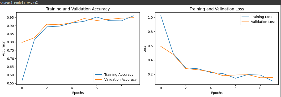
Next, visualization of graphs is performed to understand the model's performance during training. Two graphs are displayed: the accuracy graph and the loss graph for both the training and validation sets. This helps to understand how the model's performance evolves over the number of epochs (iterations) during the training process. These graphs provide a visual understanding of how the model learns from the data.

            Model Accuracy: 94.74%
            

Finally, the accuracy of the model on the validation data is printed to provide information about how well the model can predict unseen data. This accuracy score gives an indication of how well the model can generalize patterns from the training data to new data.

After training the model, its performance is evaluated using validation data. The model accuracy on validation data is then printed to provide an overview of the overall performance. Additionally, graphs of accuracy and loss on both training and validation sets are displayed to aid visual understanding of the model's performance, resulting in the following:

7. Proof of Work Results

                def predict_image(file_path):
                img = image.load_img(file_path, target_size=(150, 150))
                img_array = image.img_to_array(img)
                img_array = np.expand_dims(img_array, axis=0)  # Create batch axis
                predictions = model.predict(img_array)
                predicted_class_index = np.argmax(predictions)
                class_labels = train_generator.class_indices
                predicted_class = list(class_labels.keys())[predicted_class_index]
                return predicted_class, predictions

This function predict_image() is defined to predict the class and probability distribution of an image given its file path. It first loads the image using image.load_img() from the file path and resizes it to the required dimensions (150x150 pixels). Then, it converts the image into an array using image.img_to_array(). To make predictions, the array is expanded to add a batch dimension using np.expand_dims() since the model expects input in batches. The model's predict() method is then used to obtain predictions. The predicted class index is determined using np.argmax() on the predictions array, and then converted back to class label using the class indices obtained from the train_generator.

            uploaded = files.upload()
            
            for fn in uploaded.keys():
                predicted_class, predictions = predict_image(fn)
            
                img = mpimg.imread(fn)
                imgplot = plt.imshow(img)
                plt.show()
            
                print(f"File: {fn}")
                print(f"Predicted Class: {predicted_class}")
                print(f"Predictions: {predictions}")
            

In this loop, each uploaded image is iterated through. For each image, the predict_image() function is called to obtain the predicted class and prediction probabilities. The image is then read using mpimg.imread() and displayed using plt.imshow() for visual inspection. Finally, the file name, predicted class, and prediction probabilities are printed to provide insight into the model's predictions.

Generally, a function that takes the image path as input and returns the predicted class and probability distribution from the trained model. The image is converted into an array, expanded by adding a batch dimension, then predicted using the model. The prediction results are then converted back into class labels.

            uploaded = files.upload()
            

This code allows users to upload images for prediction. Below is an example of the uploaded image and its result:

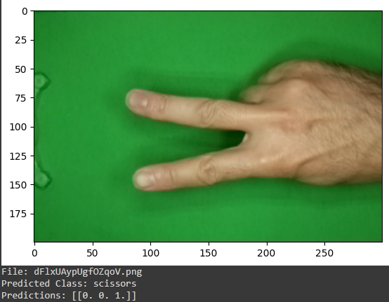
The final step involves proving the results of the model's work by predicting uploaded images. The uploaded images are also displayed for easier visual understanding. This process involves using a function to predict images, displaying the uploaded images, and displaying the prediction results from the model.

Conclusion

In this article, we have learned the steps involved in developing an image classification model using deep learning techniques. By following these steps, we can create and evaluate a model capable of classifying images of hands depicting rock, paper, and scissors with satisfactory accuracy. Hopefully, this article is helpful in understanding the concepts and implementation of machine learning models. Thank you.

To view a more detailed analysis, please refer to my complete analysis on Kaggle.

Back